3F1 Signals ad Systems Tripos Revision

$ \require{amstext} \require{amsmath} \require{amssymb} \require{amsfonts} $

Transfer Function for discrete system:

For a system to have a transfer function, it has to be linear and time invariant. That is, LTI. Stable: Bounded input gives bounded output. No poles in the right-half plane or imaginary axis.
Pulse response $\{g_k\}$ of a system G is the output of the system with input of a pulse $\delta_k$:

$ \delta_k = \left\{ \begin{array}{ll} 1, \quad k=0 \newline 0, \quad \textrm{otherwise} \end{array} \right. $

Then, the output of the system G with an arbitrary input $u_k$ would be the discrete convolution between the input $u_k$ and the pulse response $g_k$:

$ y_k = \sum_{i=0}^{k}u_i g_{k-i} = \sum_{i=0}^{k}u_{k-i} g_i $

Steady State Response of the filter $G(z)$:
- Frequency Response: If input is $\cos(k\theta)$: $ y_{ss}(k) = |G(e^{j\theta})|\cos(\theta k + \angle G(e^{j\theta})) $
- Step Response: $ y_{ss}(k) = y_k = G(e^{j0})= G(1) $
  - This is actually from the final value theorem, however, you need to prove stability of the system with this

FIR IIR Poles

For the pulse response $g_k$ if it terminates after a finite number of time steps:

$ \{ g_k\} = (g_0,…,g_n,0,…,0) $

It is FIR. It has transfer functions:

$ G(z) = g_0 + g_1z^{-1} + g_2z^{-2} +…+ g_nz^{-n} $

Otherwise it’s IIR.
This shows that all the poles of transfer function of FIR are at zero. i.e. $(z-0)=0$
And Causal system have the same transfer function. To be causal, $G(z)$ needs to be finite as $z \rightarrow \infty$, and here $G(z) \rightarrow g_0$.
Oscillation: It happens when systems have real poles on negative real axis. i.e. for $G(z) = 1/(z-p)$, the denominator: $z-p=0$ and $p<0$. For oscillation to occur, the system is IIR could not be FIR, since it will decay or grow infinitely depends on whether p larger or smaller than 1.

Stability

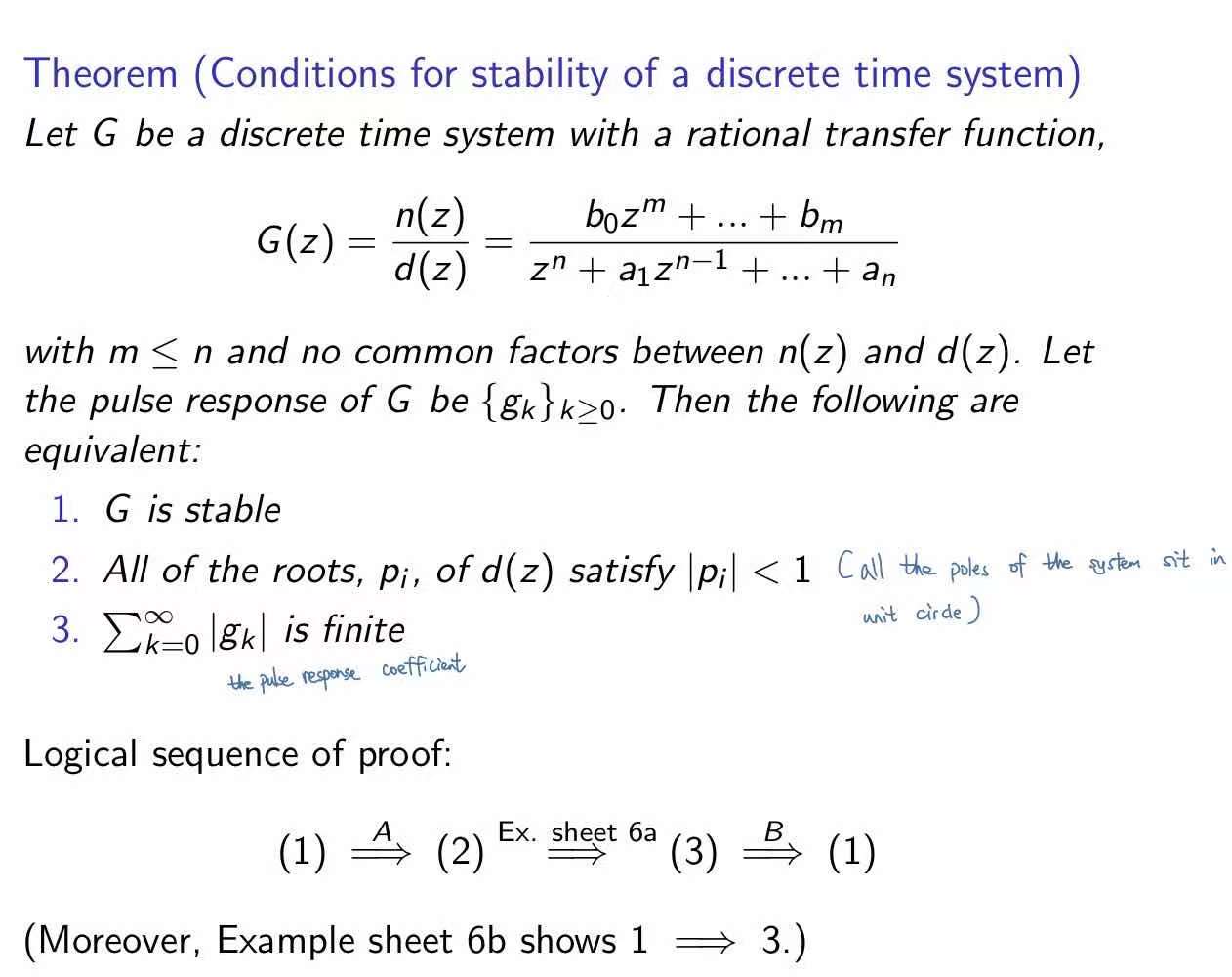
Usually, we use the second one to prove the stability from the transfer function, the pole of the denominator.

Solving Z transform

Use the data book to solve for the transfer function by forward z-transform and inverse z-transform. Remember to use partial fraction when there is two or more separable term in the denominator.

Bilinear Transform for Mapping analog filter to digital filter

Stable analog prototype filter results in stable digital filter. In continuous filter, s-domain, the poles are all in left half plane. Each of the poles map onto the points inside the unit circle for the discrete, digital filter, z-domain.

$ s = \frac{z-1}{z+1} $

Take inverse function:

$ z = \frac{1+s}{1-s} $ assume $s=\lambda + jw$, we would have $|z|^2 \le 1$

Frequency warping between analogue and digital domain.
- Analogue filter: $G_c(s)$, frequency response: put $s=j\omega$, $G_c(j\omega)$
  - Zero Frequency: s=0
  - Infinite frequency: $\infty$
- Digital filter: $G_d(z)$, frequency response: put $z=e^{j\omega}$, $G_d(e^{j\omega})$
  - Zero frequency: z=1
  - Infinite frequency: $z=-1$
- We want the response of the digital filter to be identical as the analogue filter: $ G_d(z) = G_c(s) = G_c(\frac{z-1}{z+1}) $ $ G_d(e^{j\omega}) = G_c(\frac{e^{j\omega}-1}{e^{j\omega}+1}) = G_c(j\textrm{tan}(\theta / 2)) $
- If the normalised cut-off frequency for the digital filter is $\Omega$, then the analog cut-off frequency is $\textrm{tan}(\Omega/2)$
Normalised cut-off frequency is computed w.r.t the sampling period. If sampling period is T, then the max frequency B.W. is $\omega_{MAX}=\frac{2\pi}{2T}$. Given cut-off at $f$, $\omega = 2\pi f$, the normalised cut-off frequency is $\frac{\omega}{\omega_{MAX}}\pi$
Aliasing, overlapping and Shannon theorem, the sampling frequency needs to be two times greater than the maximum frequency of the system.

Windowing and Filter Design

Inverse transform could be used to find the impulse response, and then window can be applied to take samples. Then from the sampled impulse response, the transfer function could be found by taking a z transform.
Wider window: wider window, larger sampling point N, it reduces transition band of the filter.
Computing the impulse response $\{g_k\}$ of the FIR filter: $ g_k = h_{k-N/2}w_k $
- $h_t$ is the impulse response of the ideal filter, say low pass.
- $w_t$ is the impulse response of the windowing function say Hamming or Rectangular window.
- $N$ is the number of the sampling points.
Rectangular Window vs Hamming window:
- Hamming window reduces the ripples of the final filter.
Distortion introduced by the windowing:
- The product between the ideal filter and the window corresponds to convolution in frequency.
- The convolution between the frequency domain ideal filter $H(e^{j\theta})$ and frequency domain window response $W(e^{j\theta})$ introduces distortion on the ideal filter frequency response

DTFT, Convolution and Circular Convolution

For a 11 samples FIR filter, 100 point DFT hardware, compute the response of the system to a sequence $x_k$ of 200 sample:

M=10, N=100
Process via FFT hardware of 100 requires to have the following frame: $ x_1 = [0,…,0,x_0,…,x_{89}] $ initially place extra M zeros, since the hardware is 100, put first 90 x into the first frame $ x_2 = [x_{80},…,x_{89},x_{90},…,x_{179}] $ repeat the previous M samples and add N-M (90) more samples $ x_3 = [x_{170},…,x_{179},x_{180},…x_{199},0,0,0…] $
Give the impulse response g in vector form, compute the fft for each: G = FFT(g), $X_1$ = FFT(x_1), $X_2$ = FFT(x_2), $X_3$ = FFT(x_3)
$Y_1 = G X_1$, $Y_2 = G X_2$, $Y_3 = G X_3$
then Apply IFF for each of them, the output is the last $N-M$ samples, 90 here.

Random Process

Continuous Random Process
- Defining the autocorrelation function:
$ r_{XX}(t_1, t_2) = E[X(t_1), X(t_2)] = \int\int x_1 x_2 f(x_1, x_2)dx_1 dx_2
$

$x_1, x_2$ are the values of the random process at the respective time, $f(x_1,x_2)$ is the joint PDF
- Defining the Power Spectral Density:
$ S_{X} = FT[r_{XX}(\tau)] = \int r_{XX}(\tau)e^{-j\omega \tau} d\tau $
- For SSS(Strict Sense Stationary): The probability distribution does not change over time.
- For WSS: The mean of $x_n$ is constant, independent on time. The autocorrelation only depends on the time difference.
- Mean and correlation ergodic: The WSS process’s mean and correlation function computed over the ensembles equal to the respective value computed by averaging over time:
$ E[X] = \lim_{N\rightarrow \infty}\frac{1}{2N} \int_{-N}^{N}X(t)dt $

$ r_{XX}[\tau] = \lim_{N\rightarrow \infty}\frac{1}{2N} \int_{-N}^{N} X(t) X(t+\tau)dt $
White Noise:
- Zero Mean $E[\epsilon]=0$
- $r_{XX}[m] = \sigma^2 \delta(m)$ The autocorrelation function is a delta function, means uncorrelated if $m \not= 0$
Remember that the mean-square value for a process is just the autocorrelation at $\tau=0$

Random Process with LTI system

Define input and output for the LTI system with WSS processes:

$ y(t) = h(t) \star x(t) = \int h(\beta) x(t-\beta)d\beta $

this is the continuos domain convolution

PSD relating input and output:

$ S_Y(\omega) = S_X(\omega)|H(\omega)|^2 $

$H(\omega)$ is the fourier domain transfer function

Relating PSD and autocorrelation function:

$ r_{YY}[\tau] = \frac{1}{2\pi}\int_{-\infty}^{\infty}S_{Y}(\omega)e^{j\omega\tau} d\omega $

$ r_{YY}[0] = \frac{1}{2\pi}\int_{-\infty}^{\infty}S_{Y}(\omega) d\omega $

The autocorrelation is the Inverse fourier transform of the PSD

Cross Correlation: $ \begin{align} r_{XY}[t_1,t_2] =& E[X(t_1)Y(t_2)] \newline =& E[X(t_1)\int h(\beta) X(t_2-\beta)d\beta ] \newline =& \int h(\beta)r_{XX}(t_1,t_2-\beta)d\beta \newline =& h(\tau)\star r_{XX}(\tau) \end{align} $ where $\tau = t_2 - t_1$